HP-15c’s built-in matrix feature can greatly save time and decrease the number of lines when incorporated in a numerical analysis program. I used it extensively during my Numerical Methods subjects in graduate school.
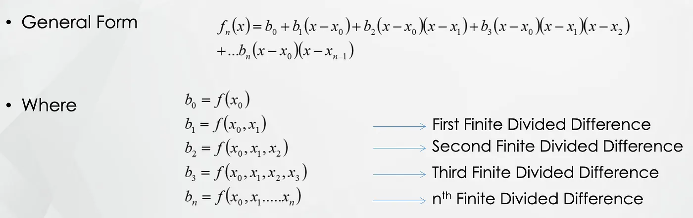
For example, to interpolate (curve fitting) using Newton’s divided difference, we can input the data, x and f(x) using the matrix functionality.
Please see below example and HP15c program:

Program Keystrokes:

   000 {             }
   001 {    42 21 11 } f LBL A
   002 {          36 } ENTER
   003 {          36 } ENTER
   004 {          36 } ENTER
   005 {       32 14 } GSB D
   006 {       44  3 } STO 3
   007 {          34 } x↔y
   008 {           1 } 1
   009 {    42 16  0 } f MATRIX 0
   010 {    42 23 11 } f DIM A
   011 {    42 23 12 } f DIM B
   012 {          30 } −
   013 {       32 14 } GSB D
   014 {       44  2 } STO 2
   015 {    42 16  1 } f MATRIX 1
   016 {    42 21  0 } f LBL 0
   017 {       45  0 } RCL 0
   018 {          31 } R/S
   019 {    44 11  u } STO A
   020 {       22  0 } GTO 0
   021 {    42 21  1 } f LBL 1
   022 {       45  0 } RCL 0
   023 {          31 } R/S
   024 {    44 12  u } STO B
   025 {       22  1 } GTO 1
   026 {    42 21 12 } f LBL B
   027 {       45  3 } RCL 3
   028 {       44  0 } STO 0
   029 {       45  2 } RCL 2
   030 {       43 44 } g INT
   031 {          26 } EEX
   032 {           3 } 3
   033 {          16 } CHS
   034 {          20 } ×
   035 {    44 30  0 } STO − 0
   036 {    42 21 13 } f LBL C
   037 {           1 } 1
   038 {          36 } ENTER
   039 {    45 40  0 } RCL + 0
   040 {          34 } x↔y
   041 {    45 43 12 } RCL g B
   042 {       45 12 } RCL B
   043 {          30 } −
   044 {       45  2 } RCL 2
   045 {       43 44 } g INT
   046 {    45 40  0 } RCL + 0
   047 {           1 } 1
   048 {    45 43 11 } RCL g A
   049 {       45 11 } RCL A
   050 {          30 } −
   051 {          10 } ÷
   052 {       42 31 } f PSE
   053 {       42 31 } f PSE
   054 {       42 31 } f PSE
   055 {       44 12 } STO B
   056 {    42  6  0 } f ISG 0
   057 {       22 13 } GTO C
   058 {    42  6  2 } f ISG 2
   059 {       22 12 } GTO B
   060 {       43 32 } g RTN
   061 {    42 21 14 } f LBL D
   062 {          26 } EEX
   063 {           3 } 3
   064 {          16 } CHS
   065 {          20 } ×
   066 {           1 } 1
   067 {          40 } +
   068 {       43 32 } g RTN
To use the HP-15c program:
How to run the program A
N f A
where N= number of data points
example: N=4
X = [5, -1, -3, 2]
Y = f(X) = [120, -6, -32, 3]

4 f A
1.000 (display prompt to enter X1)
R/S (input X1 and press R/S)
2.000 (display prompt to enter X2)
-1 R/S (input X2 and press R/S)
3.000 (display prompt to enter X3)
-3 R/S (input X3 and press R/S)
4.000 (display prompt to enter X4)
2 R/S (input X4 and press R/S)

1.000 (display prompt to enter f(X1))
120 R/S (input f(X1) and press R/S)
2.000 (display prompt to enter f(X2))
-6 R/S (input f(X2) and press R/S)
3.000 (display prompt to enter f(X3))
-32 R/S (input f(X3) and press R/S)
4.000 (display prompt to enter f(X4))
3 R/S (input f(X4) and press R/S)

display the output : (pause 3 seconds after each display)
21  f(X1,X2)  coefficient a1
13   f(X2,X3)
7    f(X3,X4)
1   f(X1,X2,X3) coefficient a2
-2   f(X2,X3,X4)
1   f(X1,X2,X3,X4) coefficient a3

and a0 = 120; the first and initial f(X1)
f(x) = a0 + a1(X-5) + a2(X-5)(X- (-1)) + a3(X-5)(X-(-1))(X-(-3))
f(x) = 120 + 21(X-5) + 1(X-5)(X+1) + 1(X-5)(X+1)(X+3)
f(x) = 120 + 21(X-5) + (X-5)(X+1) + (X-5)(X+1)(X+3) --> Perfect Fit!!!